Exploring Medicine – A Foreword

I remember clearly the first meeting I had with Steve Jameson in summer 2005. I had just returned from a regional meeting of the National Association of Advisors in the Health Professions (NAAHP) where a number of sessions had focused on the importance of having health professions advisors build partnerships with health care practitioners in the community. So, when approached by Steve I was more than glad to meet to discuss what I thought was merely an opportunity to enhance our students’ access to shadowing opportunities.

Although that original meeting has led to much greater student access to clinical experiences, then I had no idea that it was the launching pad for an innovative educational experiment in the health sciences that has deeply contributed to the academic, professional, and personal development of hundreds of students – Exploring Medicine. In our first conversations in 2005, Steve proposed to teach a course at the College of Saint Benedict/Saint John’s University (CSB/SJU) that would show students how to critically think like a doctor and how to apply the material they were learning in basic science courses to the process of clinical diagnosis.

We eagerly supported Steve’s idea and in spring 2006 Exploring Medicine was taught for the first time. Since then it has been taught every spring at CSB/SJU and more recently in the fall semester at the University of St. Thomas. Exploring Medicine is truly a gem since it allows students to critically engage in a focused and structured learning experience from a clinical standpoint. Through Steve’s interactive lectures students develop analytical skills that allow them to experience the thinking process of a clinician making a diagnosis; through the panels of healthcare professionals and guest speakers students gain an appreciation for the diversity of the healthcare field and the necessity for a team-approach in care; and last but not least, through the structured shadowing experiences provided by the class students can see how principles covered in the course are directly applied in the process of diagnosis and patient care. Indeed so many students continue to pursue the relationships they have established with clinicians in Exploring Medicine that at CSB/SJU, with Steve Jameson’s help, we established a year-long internship program at the St. Cloud Hospital Emergency Department entitled the Student Health Assistant Program. Engaging community physicians to teach at local universities pays dividends, and Exploring Medicine is the ideal platform to establish those relationships.

The uniqueness of Exploring Medicine is that it is not static – Steve Jameson is continuously editing and tailoring his presentations, creating new experiences for students, and providing novel leaning tools and settings. Since 2006 Exploring Medicine also came to include this book – it is used for the class, but many Exploring Medicine alums will also vouch for its continued value as a refresher and review tool in their further studies. More recently Steve has developed online resources that allow Exploring Medicine to be delivered in its unique and creative fashion to health professions students in any college campus throughout the country; tools that were recognized by the AAMC with its 2013 iCollaborative award in biology.

In short, Exploring Medicine is much more than a course, a book, or a set of online tools. Exploring Medicine is a unique experience that allows health professions students to directly bridge their academic background to a structured clinical setting, and to begin to experience the intellectual world as seen through the eyes of a physician. In the process of helping Steve implement his vision at CSB/SJU, I have seen hundreds of students who are now working as physicians, physician assistants, physical therapists, among others engage in their first meaningful clinical discovery in that setting. Exploring Medicine is indeed the bridge from the world of the humanities, social and natural sciences of our college campuses to the experiential setting of clinical medicine and practice.

Manuel Campos, Ph. D.

Professor of Biology, Preprofessional Health Advisor College of Saint Benedict|Saint John’s University

Preface

Choosing a career is one of the most important decisions you will make in your life. While a career in health care, and in medicine in particular, can be incredibly exciting and rewarding, the journey to that end can be an enormous physical, emotional, and financial drain. The decision to go into this field must be an informed one.

Many are enamored with the medical field and with “being a doctor” long before they know much at all about the practice of medicine. Some are told, “You’re smart; you should be a doctor.” Others simply like what they see on TV. The Exploring Medicine series of modules will primarily focus on what it is like to be a physician, but the information is relevant to all that are seeking a career as a health care professional. To make an informed decision regarding a career in medicine, you should first explore the medical field by seeing what physicians do and learn to think like a physician.

This module, and others in this series, will allow you to do just that. Starting with the very first topic, you will plunge into the world of clinical practice. There you will find patients with a variety of medical problems (based on actual cases), many with life-threatening and life changing emergencies that you will need to work through and solve in order to save your patient’s life and make them well. By the time you have finished this module you will have learned to think and problem-solve like a doctor, and you will understand the process of diagnosing and treating disease.

The medical model is all about diagnosis and treatment of disease, and in order to understand that you have to understand pathophysiology. Pathophysiology is the study of disease. The pathophysiologic process of a disease is the series of events that take place and conditions that develop that result in a particular disease. In order to treat disease, the physician must understand something about the pathophysiologic process that led to the development of that disease. By going through the systems based modules you will gain insight into the thought process physicians use to diagnose and treat disease, and how they help patients to become well. Each system based module begins with a general overview followed by a discussion of the pathophysiology of a particular disorder: e.g. the Respiratory module reviews anatomy and physiology of the Respiratory System, then goes into a discussion regarding the cause of asthma and its treatment. Other modules, like Social Determinants of Health, focus on wellness as it relates to society, social factors, and public policy. Exploring Medicine modules were made for the students that have taken biology, chemistry, sociology, psychology, and other science courses, and wondered, “Why do I have to learn this stuff?” These modules apply the student’s science knowledge to the real world by making correlates to clinical medicine.

Books have been written on what will be small elements of the Exploring Medicine modules, so we obviously cannot comprehensively cover every topic. The authors have distilled a massive volume of material down to several manageable lessons. Despite this editing, the amount of subject matter may still seem intimidating at first, but that is not the intent of the authors. Do not get stressed or anxious. The focus of these modules will be on general principles and concepts. In order to transition from simple anatomy and physiology to treatment of disease, for example, we must streamline our approach in order for the reader to get some appreciation of what it is like to be a physician. The following module will take you, the medical enthusiast, through a very narrow slice of medical training: from medical school, to residency training, to clinical practice. Armed with your newly found knowledge, you will be able to make clinical decisions based on true-to- life patient scenarios and help your patients become well or stay well. If you find this process compelling, as the authors do, then you may seriously want to pursue the exciting field of medicine.

Introduction to the Chapters – Life and Death, Homeostasis and Equilibrium

Death is not the enemy but occasionally needs help with timing. – Peter Safar, M.D. The “Father” of CPR

What is life? That may seem like a metaphysical question, but it’s actually not. It is a very real question for those that provide medical care, but the answer can be surprisingly complicated. As a physician, physician assistant, nurse, or nurse practitioner, you will likely have many occasions where you will be dealing with patients as they look to cross that line from life to death. In the following chapters we will discuss a variety of pathophysiologic processes that will alter the normal function of the human body.

Before we delve into specific disease processes, though, let’s take a look at a more fundamental principle of human physiology and how a disruption of normal processes can lead to chaos, i.e. entropy, on a microscopic (actually molecular) level and to death on a macroscopic level.

The human body is a complex network of systems that operate in unity to keep us alive and active. In order to maintain normal function the body seeks homeostasis and defies equilibrium. Cellular reactions take place under very specific conditions: a narrow range of pH, the correct concentrations of particular ions, proper amount of substrates, etc. Homeostasis is the set of conditions that the body establishes and maintains in order to function properly. It takes energy to maintain this homeostasis. This energy has to be consumed in the form of chemical bonds contained in the food we eat, converted to a usable form, transported throughout the body to all of its cells, and metabolized into a form of energy the cells can use: ATP. The wastes of these reactions then have to be removed. It is a complex network of integrated systems that accomplishes all of these tasks.

In Exploring Medicine, we will look at four of the body’s integrally related physiologic systems (Cardiovascular, Respiratory, Renal and Integumentary) as examples of how the body maintains homeostasis. We also explore what can happen when these systems fail, and what we, as medical care providers, do to restore normal function and reverse the process of dying. All of the chapters have questions to answer along the way and challenging scenarios to solve at the end of each chapter. Answers to these questions and further elaboration of concepts are in the appendices near the end of the book. In the chapter on Evidence Based Medicine, we will discover how the medical literature helps to guide a physician’s clinical practice. As you strive to learn more about the field of medicine, remember the words of Hippocrates (the final line of the Hippocratic Oath), “May I always act so as to preserve the finest traditions of my calling and may I long experience the joy of healing those who seek my help.”

Evidence Based Medicine Unit Quiz

This is an open book test. You can click here to open the lesson in a new tab/window to review the lesson as you take the quiz. If you close the quiz you will have to start all over with a different set of questions. You need to achieve a score of 90% or greater in order to obtain the certificate of completion.

Please ensure you have enough time to complete the entire quiz at one time.

An Interesting Caveat

Linus Pauling, who earned Ph.D.s in both chemistry and math, is considered one of the greatest scientists of all time. He won many distinguished scientific awards including the Nobel Prize in chemistry (in 1954). Dr. Pauling is credited with the wonderfully poignant quote that starts this chapter; “Facts are the air of scientists. Without them you can never fly.” Dr. Pauling, however, failed to heed his own advice in the twilight of his career and let personal convictions cloud his scientific judgment. After making enormous strides in the fields of chemistry and molecular biology, Dr. Pauling’s interests turned to a different direction: the field of medicine. Dr. Pauling came across studies, and personally experienced anecdotal evidence, which seemed to reveal some benefit in using vitamins to aid healing. In his own battle with kidney disease he utilized vitamins, including vitamin C. At that time, vitamins were mostly used to treat deficiencies from lack of dietary intake. Linus Pauling became convinced that high dose vitamin C was beneficial in treating a variety of ailments, including the “common cold.” He based his belief on a variety of anecdotes, including his personal use, and a few studies with inadequate methods (small numbers and suboptimal control groups). Emerging evidence, including large controlled randomized trials, began to discount Dr. Pauling’s assertion of the benefit of high dose vitamin C for the common cold. Instead of being open minded to this new and convincing information, Dr. Pauling tried to discredit the researchers and their studies. Despite mega-evidence against mega-dose vitamin C, Linus Pauling held to his conviction of this therapy’s efficacy. He slowly became marginalized in the medical community and the impact of his earlier great works became eclipsed by the vitamin C controversy. The point of this lesson is that even a man of science as great as Linus Pauling can be drawn to believe something is true just because he believes it to be true. Convictions are a powerful force and can blind one from the truth. The famous Russian author Leo Tolstoy (author of “War and Peace”) considered one of the greatest writers of all time, once said (in 1894): “The most difficult subjects can be explained to the most slow-witted man if he has not formed any idea of them already; but the simplest thing cannot be made clear to the most intelligent man if he is firmly persuaded that he knows already, without a shadow of doubt, what is laid before him.” In other words, keep an open mind and be prepared to change your opinion regarding patient therapies as new studies shed light on old treatments. When faced with a controversial situation in medicine, ask yourself, “am I a person of science or simply someone with a strong conviction.”

Other Clinical EBM Scenarios

The following scenarios are designed to walk the future physician through a variety of real life situations that highlight various statistical challenges in the literature. Read the introduction closely and work through the scenario to ultimately decipher the data.

Review of Case Scenario

Patient encounters are not always simple and straightforward. Not uncommonly physicians will spend time using science to dispel myths, misconceptions, and references to anecdotes. This patient has presented with a preconceived notion that she has what a friend had (or may have had): a headache related to Lyme disease. The patient agrees to be tested for Lyme disease ahead of any treatment for this disease, and in fact her test is found to be negative. The patient returns to your office to discuss the results and reminds you that the Lyme test is not 100% accurate.

In order to discuss the probability of this patient having Lyme disease, we have to first determine the probability prior to running the Lyme titer: i.e. determine the prior probability as is done with Bayesian analysis. Since the only symptom she is presenting with is headache, you rationalize with her that of all patients presenting with headache, it is unlikely that more than 5% of them have Lyme disease. She agrees with this assertion and you agree to use 5% as a very high potential estimate of patients with Lyme related headaches. With that in mind, you create a 2 X 2 contingency table with a prevalence of disease of 5%: that means that there is one patient with disease for every 19 patients without disease. Using the Sn and Sp from the introduction of this case as 80% and 90% respectively, the 2X2 table can be produced as follows.

This means that even if 5% of all patients presenting to the clinic with headache have Lyme disease (likely a vast overstatement of the number of headache patients with Lyme), there is only a 1% chance that the diagnosis of Lyme disease was missed in this patient, not 20% as she was imagining. Armed with this knowledge, you choose not to start the patient on a course of antibiotics but instead seek out the real cause of her headaches and try a different therapy. She agrees with this plan.

Conclusion:

Everyone wants to be healthy, and patients will come to you, as a physician, for advice on how to get well when sick, or how to stay well when not sick. It is human nature to want a pill or procedure to fix everything: think of the medications and surgery available to “cure” obesity, or all of the options available to treat low back pain, or elevated cholesterol levels. Many people strive for a “natural” cure for their ailments. Before you recommend a medication or other therapy for your patient, be certain that the course of treatment recommended is backed up by solid evidence of benefit in the medical literature. Do not fall victim to believing in a particular therapy because it is trendy or because there are a smattering of anecdotal reports. Medicine is not a religion. It matters not what you “believe” in but what is statistically shown to be effective by good research studies. Be a person of science and not simply someone with a strong conviction. Learn to objectively analyze data and draw the conclusion that best suits the needs of your patients. Those conclusions will change with time, so be prepared to adapt as new studies prove old therapies to be wrong. Evidence based medicine needs to be the foundation of your medical practice.

Statistical Terms and Concepts Used in the Treatment of Disease, Statistical Significance, and Bayesian Analysis

Explanation of Statistical Terms and Concepts Used in the Treatment of Disease:

NNT and NNH:

A contemporary and practical means of assessing the benefit of a particular drug, procedure, or other therapy, or its potential risk, is through the use of a statistical measure called the number needed to treat (NNT). NNT is the number of patients that need to receive a particular therapy until there is a change in outcome in one patient: either good or bad. When we refer to the positive outcome or “benefit” of a particular therapy, this is the NNTB: number needed to treat until we are likely to see one patient receive benefit from the therapy. When we refer to the negative outcome or “harm” that occurs to a patient as a result of the studied therapy, this is the NNTH: number needed to be treated until we are likely to see one patient harmed as a result of the studied therapy. These terms may also be abbreviated simply as NNT and NNH.

To calculate the NNT or NNH we must first determine the absolute benefit or risk of a particular therapy. For NNT specifically, we first need to calculate the absolute risk reduction (ARR) for a therapy. As always, concepts like this are best learned by looking at examples, so let’s imagine a simple study such as this. Let’s say the drug X is a new chemotherapy agent that treats malignant melanoma. When tested blinded and randomly in a population of 200 patients, the placebo drug resulted in no cures from this cancer in the 100 patients it was tried in (all patients died). In the 100 patients that received drug X, 50% of patients survived with no trace of cancer. The ARR equals the control event rate (CER, representing the proportion of patients that died in the control group, i.e., those that received the placebo treatment), minus the experimental event rate (EER, in this case representing the proportion of patients that died that received the study drug):

ARR= CER-EER

ARR= 100/100- 50/100=50/100=1/2

ARR = 0.5 or 50%

NNT is the inverse of the ARR:

NNT= 1/ARR

NNT= 100/100-100/50=100/50

NNT = 2

This means that 2 patients would need to be treated with this new drug before we would expect one to be cured of cancer. The higher the number, the less effective the therapy is.

In turn, NNH indicates the likelihood that a specific therapy will harm a particular population of patients. Using this same example, let’s say that 5 patients in the treated group died as a result of therapy with drug X and no patients died during therapy with placebo. To calculate NNH (aka. NNTH), we have to calculate the absolute risk increase (ARI) of a particular therapy. ARI is the opposite of ARR so the values used to calculate ARI are the reverse of those used to calculate ARR. ARI is calculated by taking the proportion of patients harmed in the experimental group (where there was more harm done to patients) and subtracting it from those harmed in the control group.

ARI=EER-CER

ARI=5/100-0/100=5/100

NNH = 100/5 = 20

This means that you would expect one person to die as a result of receiving the chemotherapy drug X for every 20 patients treated with this drug.

Some investigators and clinicians like to look at the proportion of risk vs. benefit of therapy. You can do that in the following manner by simply dividing the NNH by the NNT. If the quotient is greater than one, then there is more benefit than harm. If the quotient is less than one, there is more harm than benefit. In our example the risk/benefit ratio of using this new chemotherapy drug is:

NNH/NNT=20/2

NNH/NNT=10

This means that your patients are 10 times more likely to get benefit from this therapy than be harmed by it. The ideal NNT would be 1. That means that every patient treated with a particularly therapy received benefit and those not treated did not get benefit. There are few, if any, therapies like this. For further explanation about NNT, and for more examples and calculations, see appendix 5a.

Relative Risk or Risk Ratio (RR) and Odds Ratio (OR):

RR and OR are statistical measures commonly used in medical literature to analyze outcomes of 2 groups: usually a treatment group vs. a non-treatment group. These methods can also be used epidemiologically to determine the risk of developing a disease when exposed to certain risk factors: in this case we compare the development of disease in the exposed group vs. the non-exposed group. RR and OR data are very practical and useful when counseling patients regarding particular therapies or exposures.

RR and OR values tend to “track together.” That means that as one goes up, indicating, for example, a more useful treatment, the other will go up. Their values, though, are different because of the way they are calculated. RR is a “relative” value so it is a percent. It is calculated, in simple terms, by taking the number of patients in the “group of interest” (e.g. all of those that were successfully treated) divided by all studied patients (all treated patients, whether

they successfully treated or not). If, for example, you found that migraine patients had relief of their headaches 80 percent of the time with drug A and only 20% of the time when using a placebo, the RR would be 80/20 or 4. That means that you are 4 times more likely to have your headache controlled if you use drug A than if you use placebo. The calculation looks like this:

RR=(80/100)/(20/100)=80/20=4.0

Odds ratio, on the other hand, is not a percent but is “odds.” That is to say, it is the chance of an event happening vs. all other possible outcomes. Using the same example above, the odds that drug A will be useful in the treatment of headache is the odds of a good outcome with the drug over those without a good outcome, divided by those not treated that had a good outcome over those not treated that did not have a good outcome. The calculation would look like this:

OR=(80/20)/(20/80)=4.0/0.25=16

This means that the odds are 16 to 1 (or 16 times greater) that you will have improvement of your headache if you use drug A vs. placebo.

Interestingly, as the effect of treatment becomes less significant, the value of OR begins to approach that of RR. Let’s say in another study only 80 out of 1,000 received relief of headache with drug B vs. 20 out 1,000 with placebo. What would the calculations of RR and OR look like?

RR =

OR =

Answer:

RR=(80/1000)/(20/1000)=4.0

OR=(80/920)/(20/980)=4.3

Notice how the values of RR and OR are nearly the same when there is a low prevalence of an event.

When comparing two therapies, e.g. therapy A vs. therapy B, if the RR or OR turns out to be 1, then there is an equal chance that the patient will get same benefit whether they receive therapy A (the study “subject” therapy) or therapy B (placebo or perhaps the current conventional therapy). “1” is considered the null value, meaning there is no difference between these therapies. Using our example above, a value greater than 1 indicates that there is some benefit to treatment with the “subject” drug (drug being tested). If you were assessing a drugs ability to decrease the risk of heart attack, then a value less than 1 would indicate a negative correlation between taking this drug and a heart attack event. In this case, a value less than 1 would be good, and would indicate a benefit in using this drug to prevent heart attacks.

When used epidemiologically, RR and OR tell us the chance of developing a disease based on exposure to a particular agent: take patients that are smokers vs. non-smokers and their risk of developing lung cancer. If the value of RR or OR is greater than 1, then it is more likely that smokers will develop lung cancer. The higher the value of RR or OR, the greater the risk is of developing lung cancer in smokers vs. non-smokers. For more explanation of the concepts of RR and OR, please see appendix 5a.

Statistical Significance:

Statistical significance, simply put, is the acceptance that something occurred because of something other than random chance. That doesn’t mean that we’ve proven that random chance didn’t occur, but that it is so unlikely that the finding was random that we accept the fact that it isn’t. Let’s look at an example. Say that a man shows us that he has two coins. On inspection of the coins, we see that one of them is a normal coin with a heads and tails side, and the other is a two headed coin – has identical sides with heads on both sides. He places the coins in a hat and pulls one of them back out. He begins to flip the coin and then show us the result. On the first flip, it comes up heads. Is this the two headed coin? We can’t really say at this point since there was equal chance that it could have been heads or tails. He flips it again, and it comes up heads. At this point we still can’t say it is a two headed coin since this could certainly happen by random chance as well. He flips it a third time, and heads comes up again. We are now becoming suspicious that he is flipping a two headed coin, but at what point are we going to accept the fact that this is a two headed coin? At what point are we going to reject the null hypothesis that this is a normal coin, four heads thrown in a row, five, ten? The fact is that all of these scenarios could have been the result of using either a two headed coin or a coin with both a head and tail side. At what point, though, is the chance such that we would accept the fact that a two headed coin is being flipped? This is the basis of statistical significance, or more properly statistical inference (drawing a conclusion based on the statistical results of a study).

Investigators perform studies to determine if a study subject is better or more effective than placebo or some current gold standard. The assumption going into the study, however, is that there is no difference between the study groups; this is called the null hypothesis. Statistical significance is simply a mathematical way of determining how likely it is that 2 groups are the same (or aren’t the same). When a difference between groups is found in a study, investigators have to determine if that difference is due to random chance or if it is because there is truly some effect imposed by the intervention (the study subject) of one of the groups.

The statistical difference between groups is defined (by convention) as the mathematical point at which the likelihood of finding the difference discovered is so small that we agree to believe it probably wouldn’t have occurred by chance alone. When it is that unlikely, traditionally at a 5% chance level, we agree to reject the null hypothesis and assume that the two groups are not identical and that the study subject did in fact have a statistically significant effect. In other words we acknowledge that it is unlikely that the difference between the groups is due to chance alone. Further, this means that there is a “real (mathematical) difference” between the groups and that the study subject accounted for that difference. Statistical significance is usually measured in one of two ways in medical literature: either p-values or confidence intervals.

p-value (p):

As a more traditional means of determining statistical significance, a p-value is the point at which statistical significance is defined: typically at 5% (p = 0.05). Going through the calculation of the p-value is beyond the scope of this course, but understanding it conceptually is necessary when reading medical literature. When doing a statistical analysis between two groups, we want to know if there is a difference between these groups; in this case, we want to determine if there is a statistical difference. Our assumption, when looking at these two groups, is that there is no difference. That again is our null hypothesis. If we find that we have met a particular statistical threshold, then we reject the null hypothesis and accept that there is a difference. The highest value that “p” can have is 1. That means that the two groups are absolutely identical (something that rarely happens since random chance typically gives some variation between groups), and we fail to reject the null hypothesis. In fact for any p-values greater than 0.1 there is insufficient evidence to reject the null hypothesis, and a value between 0.05 and 0.1 is considered weak evidence to accept an alternative hypothesis. When the p-value gets to a point at which there is a 5% or less chance that the difference between two groups occurred by chance alone, at p = 0.05 or less, then we accept that there is likely a real difference between the groups and we reject the null hypothesis. At a p-value less than 0.01 there begins to be strong evidence for an alternative hypothesis. Remember that statistical significance assumes that there is neither bias nor confounders and that the difference is due solely to the study subject.

To illustrate p-value cut-offs, let’s imagine that a study was performed to compare the use of ginseng and the use of metformin in the treatment of type 2 diabetes mellitus. 1,000 patients were enrolled in the study, 500 received ginseng root and 500 received placebo. Fasting blood sugars (morning serum glucose levels before eating) were obtained and the results achieved are reflected in this illustration.

Notice that the ginseng seems to be showing effectiveness in lowering blood sugar levels in these diabetic patients. A statistician, though, calculates the p-value for this study at p = 0.47. What can we conclude from this data? In the ginseng group, the average blood sugar is lower than it is in the placebo group. Because of that, should we adopt the practice of giving ginseng to patients to control their blood sugar? The question is, is this result significant? In this case, do we, as medical providers, consider this result statistically significant?

Before we answer those questions, let’s take a look at another fictitious study. This time we are going to compare the use of metformin (a conventional therapy for diabetes) to placebo in another study of 1,000 patients with type 2 diabetes mellitus. In this study, 500 patients receive metformin and 500 receive placebo. The same fasting glucose data are obtained, and the results are illustrated in this graph.

A statistician calculates the p-value here to be p = 0.01. What can we conclude from this data?

When there is a large overlap of values for the subject group and control group, as in the ginseng example, that indicates that many of the patients in the control (placebo) group had a similar outcome as those in the treatment group. The fact that the p-value is much greater than 0.05 in the first example indicates that the treatment (study subject) did not have an accepted statistically significant impact on the outcome and therefore it is very possible that the result achieved (a small difference in post-prandial glucose) happened by chance alone. In the metformin study, where the overlap of results is small, the p-value is also very small and it is unlikely that the result achieved was by chance. We should, therefore, strongly consider, given this data, using metformin for the treatment of type 2 diabetes mellitus over the use of ginseng. Note that this study did not address the use of ginseng in combination with metformin so we cannot jump to the conclusion that using the two of them together would result in additional benefit over using metformin alone.

Confidence Interval (CI):

In contrast to the p-value, the CI gives a range of values within which the true result is likely to reside. More specifically, if the same study were to be performed 100 times, we would expect the “true result” to be in the range of all of the CI’s generated, 95% of the time. In medicine, we use the 95% confidence interval, so there is a 95% chance that the “true” result lies within this interval. Doing an actual calculation of CI is beyond the scope of this discussion, but let’s again discuss this concept using the ginseng and metformin examples. Let’s imagine that our statistician calculated the 95% CI’s for the ginseng and placebo study to be as depicted in the bar graph below.

Notice that the confidence intervals are depicted on either side of the “point value,” which is the mean glucose level as found in this fabricated study. The 95% CI for the placebo group overlaps with the point value of the ginseng group so this tells us that the difference between these groups are not statistically significant and we cannot reject the null hypothesis.

Let’s now look at the metformin study and imagine that the following bar graph is produced as the statistician calculated the CI’s depicted here.

As you can see, there is no overlap of the confidence intervals for the placebo group with the point value the metformin group and therefore this does indicate a greater than 95% confidence that we can reject the null hypothesis and accept that metformin was responsible for a significant change in blood sugars in this population of patients.

In clinical studies, CI’s are not only used when comparing mean averages but also commonly used when evaluating ratios (e.g. risk ratios and odds ratios). In these cases there would be a particular likelihood of an outcome then a stated CI within which the real result is likely to reside. For example, the odds ratio (OR) of therapy A being better than therapy B could be written as OR 6.06, 95% CI 5.96 – 6.16. Therapy A, in this case, may in fact be better than B because the lower end of the CI is moderately high and well away from a value of 1.00 (which is neutral). If on the other hand, when comparing therapy A and therapy B, you observed that the statistical analysis revealed a RR of 1.25, 95% CI 0.75 – 1.75, this would indicate that it is unlikely that there is a difference between the two therapies since the confidence interval includes the value 1.00 (neutral for RR) in the range of the CI. If the value 1 is not within the 95% CI, then there is some degree of significance to this measure. For Odds Ratio, Risk Ratio, and Likelihood Ratio, if the value 1(the “null” value) is within the 95% CI, then the result of the study is not statistically significant (we cannot conclude that the subject studied had an effect the outcome to a statistically significant level and the null hypothesis cannot be rejected).

p-value vs. CI:

As stated, p-values give a specific point cut off (normally at 0.05) beyond which statistical significance is defined. CI’s give a range of values within which the “true result” is likely to reside. Researchers are utilizing confidence intervals more, and journals are demanding their use, because they give a better indication of the reliability of the result. The advantage of the CI is that if the CI is narrow, the study has good precision. If the CI is wide, this indicates less precision in the study and results that are less reliable, even if there is statistical significance by a p-value of less than 0.05. A wide CI means that there is a greater likelihood of the result happening by chance alone and you (as a clinician) would be less likely to accept the study as definitive, and thus less likely to choose this test or therapy for your patients. Larger study populations typically yield narrower CI’s and thus more reliable results.

Statistical vs. Clinical Significance:

The English definition of “significant” is to be important. To achieve statistical significance in a study doesn’t necessarily mean that the result is “important,” it simply means that the result didn’t likely happen by chance alone. A statistically significant difference may in fact not be clinically meaningful at all. There are three things that you want to know about the result of the study once it has achieved statistical significance:

Is the result of the study meaningful?
Is the result generalizable? In other words, does this result apply to the patients that I treat and can I use this intervention and achieve the same result?
Is the study free of bias?

Let’s look at an example:

Investigators studied the effect of using high dose epinephrine (10 mg) in cardiac arrest vs. standard dose (1mg). Results of studies revealed that patients had a significant improvement in “return of spontaneous circulation” (the heart generated enough of a blood pressure that a pulse could be felt, at least transiently). High dose epinephrine was then incorporated into the American Heart Association ACLS (Advanced Cardiac Life Support) algorithms. Good news for cardiac arrest patients, right? Actually, as it turns out the rate of death and permanent disability was found to be the same for the 2 groups, so the important clinical effect was not improved at all (in fact the data suggested a trend toward more patients surviving in a permanently vegetative state: probably a more negative outcome). The use of high dose epinephrine was subsequently abandoned because there wasn’t a good meaningful outcome for patients.

Another clinical example is that of a study that found that a certain spinal manipulation resulted in a statistically significant increase in the white blood cell count in blood (Brennan, et al). This study was then used as evidence, by some practitioners, that spinal manipulation helps fight infection. Is that a valid conclusion? The study didn’t measure any kind of disease outcome, and the increase in WBC count was a trivial difference and meaningless since both values (before and after) were within a normal range. In other words, the statistically “significant” difference was not a truly significant or important difference clinically for the patient.

Benjamin Disraeli, a 19th century British Prime Minister, once said, “There are three kinds of lies: lies, damned lies, and statistics.” Regardless of what data a study shows and no matter how statistically significant the results are, one must always consider the clinical importance of a test or therapy that is recommend for a particular patient.

Bayesian Analysis:

As stated previously, Bayesian analysis is a form of deductive reasoning. It requires that the clinician establish a pre-test probability regarding a particular condition before applying a specific test to aid in the decision making process. Once the pre-test probability, or “prior probability,” is determined, the clinician then selects a test to run that will help confirm or disaffirm, for example, a diagnosis. The likelihood ratio, for example, of that chosen test’s accuracy (based on the best estimate from the literature) is applied to the pre-test probability and a post-test or “posterior probability” is determined. Let’s illustrate this with an example.

Clinical scenario: Let’s say that we discover in the medical literature that EKG’s, under usual conditions, are known to be 80% sensitive and 90% specific for determining the presence of a heart attack (a myocardial infarction or “MI”) in patients with chest pain. You evaluate 2 patients that present to the emergency department with chest pain. In the first case the nurse asks you to evaluate a 19 year old man with a sharp chest pain that came on after eating a spicy burrito. In the second case the nurse asks you to evaluate a 65 year old man who developed chest pressure while shoveling snow. Your first test in each case is an EKG, which the nurse gives you as you begin to evaluate the patient, because it is the policy in your emergency department to do an EKG on anyone with chest pain. In each case the EKG is found to be “within normal limits” or has no findings to suggest a heart attack by conventional criteria. What do you do in each of these cases? Think this through before reading on.

To determine a posterior probability, your conclusion based on the data available, you combine the prior probability with the likelihood of your test result being accurate. This can be done by applying numbers (typically in the form of percentages) but the data is subjective anyway so let’s do what is commonly done in practice and use generalities. In the first case, the 19 year old, your prior probability of a heart attack is very low. Combine that now with a “negative” EKG (LR- is 0.22 when calculated, which is reasonably good, but not great), and the posterior probability indicates that it is exceedingly unlikely that the 19 year old is having a heart attack. Your work-up is essentially done regarding heart attack, so you can now focus on another potential cause of this patient’s chest pain (consider perhaps reflux of acid into the esophagus – “GERD” – otherwise known as gastroesophageal reflux disease, in the differential diagnosis, or, say spontaneous pneumothorax).

In the second case, however, a 65 year old that develops chest pain while shoveling snow is highly likely to be experiencing chest pain related to his heart. Because your prior probability is very high, even a negative EKG (with a LR- that argues against MI) does not rule-out disease: your posterior probability is still high and you are still suspicious of a heart attack (or heart related chest pain). A positive EKG (one that shows evidence of an MI), though, would essentially rule-in disease since the prior probability is high and the LR+ (calculated at 8) is highly suggestive of MI. In this case, even with a normal EKG, your patient still needs further evaluation before you can say he is not having cardiac chest pain or a heart attack.

In clinical practice Bayesian inference is commonly performed by the physician intuitively. It is, however, performed with an understanding of the strengths and limitations of tests being ordered. With a firm knowledge of the current medical literature and clinical experience, physicians find that using Bayesian analysis works very well.

Background and Key Statistical Terms

Incorporating statistics into the review of medical literature introduces a wide range of complex topics. In this chapter we will take a broad look at how to analyze data in clinical studies and adapt the information to the practice of medicine. There will likely be a lot of new terms for you to add to your lexicon. The goal of this chapter is to be comprehensive but in a superficial manner so as not to overwhelm the reader. This chapter is a primer for evidence based medicine and statistical measures associated with this. You are not expected to become a statistician but you will be expected to become familiar with the common terms used in medical studies so you can read health care literature with a degree of confidence. A variety of examples will be used to clarify more easily the various terms and concepts. These true to life clinical scenarios are fabricated but generally represent information that is currently in the medical literature. The examples created are designed to keep the calculations simple and the concepts straightforward.

Evidence based medicine:

Using the best scientific information available to do what is currently shown to be most effective for your patient’s needs is evidence based medicine (EBM). In order to get this information, studies are performed to determine if a test or therapy is effective. To determine which study results are valid, we utilize statistics. A limited knowledge of statistics is needed to render a reasonable interpretation of the medical literature. Evidence based medicine is science, not religion; it matters not what you “believe” but what evidence there is to support your decision making.

So how do statistics facilitate decision making? By doing a statistical analysis on a study, one can classify subjects: e.g. divide patients into groups of “responders” and “non-responders.” Using statistics, one can then predict the likelihood of how patients with similar conditions will respond (e.g. to a particular drug, procedure, or other therapy). Statistical significance is a measure of whether or not the results of a study are valid or if the events that occurred could have happened simply by chance. Anecdotes in medicine are individual events that occur that seem to affect someone’s outcome, and they are often something quite impressive; for example, one might say, “high dose vitamin C cured Tommie’s cough.” How do we know that vitamin C played any role in making Tommie healthy again? How do we know that Tommie wouldn’t have just gotten better on his own once his immune system wiped out the offending pathogen (likely a virus)? Did Tommie need Vitamin C? Did he need “high dose” vitamin C? We learn the answers to these questions by performing scientific studies on populations of patients that are sick like Tommie and then giving some of them high dose vitamin C and some a placebo (a pill with no vitamin C or any active substance). Until high dose vitamin C is shown to be significantly better than placebo we cannot say that there is scientific evidence supporting its use in this circumstance. Late night infomercials are full of anecdotes which are presented as scientific facts. What the producers of these infomercials are really doing, however, is preying on the naiveté of the general population. We should all be Missourians (the “show me state” people) and say, “show me” the data. Be reasonably skeptical of information you receive and look for evidence to back up others’ assertions.

There are literally thousands of medical studies being performed at any given time. As a practitioner, you will receive a barrage of information from various sources telling you how to alter your practice. Sorting out this information can be difficult. Knowing what makes a good study is a good start, because you can toss aside any study that wasn’t performed well.

A good study should:

Have large numbers
Possess a relevant subject
Be controlled
Be randomized
Be blinded
Be well planned
Show good methods with specific details
Present data accurately with good statistical analysis

We’ll go through these points one at a time:

1) Size: The larger the population a study involves, the less likely the result it achieves will be due to chance alone.

2) Relevance: It is necessary to study a subject that is relevant to its intended application in serving a population of patients; this is a property known as external validity. There is no point studying something that is not useful. I (SJ) personally learned this the hard way. I studied the effect of using intravenous (IV) calcium prior to using another IV drug, verapamil, in the treatment of patients with PSVT (a type of rapid heart rate). Verapamil was known at the time to be very effective at treating PSVT, but it caused hypotension in a large proportion of patients. Pre-treating patients with calcium had been shown anecdotally to be effective in preventing hypotension, so I decided to study it in a blinded, controlled manner: calcium pre-treatment prior to verapamil vs. verapamil alone (the control group) in treatment of PSVT. My results, over a two year period, were favorable, but I performed the study at a time that a new drug, adenosine, was coming on the market. Adenosine was safer, more effective, and faster acting than verapamil. My study became irrelevant in the eyes of the medical community and received little attention and was not accepted for publication in a journal: a lot of work seemingly for nothing and another life lesson learned.

3) Controlled: In order to determine if one therapy is better than another, one must have a control group with which to compare. It would be virtually meaningless, for example, to cite a survival rate of a particular therapy (e.g. a new medication) without comparing it to a control group: e.g. placebo, another comparable treatment (e.g. the current accepted treatment), or a comparable historical population.

4) Randomized: Another attribute of a good study is that it needs to be randomized, and the randomization must be pre-determined. If the investigator chooses which subgroup receives a particular treatment based on any method but a pre-determined randomized protocol, bias can be introduced, and the study results are less valid.

5) Blinded: Another anti-bias measure used is “blinding”. The ideal blinded study is one in which neither the patient nor the investigator knows who is getting the investigational treatment vs. who is getting the control; this is the so called “double blind” study. If one of the parties is aware of the fact that they are getting a particular treatment, the results can be distorted.

6) Well planned: A good research study should be planned and carried out in such a way that the correct population is studied, that the study goes for the appropriate amount of time, and that the study is carried out in such a way that study groups are as similar as possible except for the different therapies that define the study groups.

7) Good methods: The method section of an article is where the investigator clearly delineates how the study was performed. If the method section does not, for example, give information as to whether the study was randomized, blinded, and/or controlled, one must assume that it wasn’t, and the study results carry much less validity.

8) Accurate data and proper statistics: Investigators must show that outcomes are properly measured. They must state whether study results are statistically significant or not. While statistical significance may be considered the “holy grail” by researchers, the lack thereof does not necessarily imply a failed study. It is often of great benefit to know that there is no difference between two study groups (i.e. to accept the null hypothesis). Many myths are dispelled in this way (e.g. high dose vitamin C’s efficacy in treating the common cold). Another detail that investigators must include is the analysis of the study data. On occasion investigators will statistically analyze a subgroup of a study and not the entire study population. It is okay to do this if it is planned prospectively (before the study begins). If an investigator, however, retrospectively analyzes a particular subgroup in an effort to find statistical significance, this is called “data snooping” and typically reflects a bias on the part of the investigator and thus makes the study results less reliable.

Key Statistical Terms in Medical Literature:

Scientific Method = The analysis of data that is collected through the appropriate sampling of a population, thus yielding the highest likelihood that the conclusions drawn are valid.

Investigational Study or Clinical Trial = The research of a particular drug, test, or procedure versus placebo or a known conventional therapy/test in an effort to determine the relative value of the two modalities.

Investigational Subject = A drug, test, or procedure that is getting investigated and being compared to the gold standard: e.g. the investigator could study the utility of a new rapid test for “Strep throat” and compare it to a gold standard, such as a throat culture.

Gold Standard = The accepted test or therapy that is considered definitive. The gold standard is what the investigational subject is compared to: e.g. the gold standard for Strep throat testing could be a throat culture, which takes 2 days to run, compared to an investigational subject, such as a “rapid” Strep test, which gives a result by a different method in just 15 minutes. A study is only as good as the gold standard it uses. It is difficult to have a perfect gold standard, e.g. where the presence and absence of disease is identified 100% of the time, but we have to sometimes accept a gold standard that is less than perfect. In our strep culture example, it may be the case that the swab specimen is not always adequately collected and therefore the strep organism is not swabbed from the surface of the tonsil when it is actually present. In this case, even by gold standard, the patient would be diagnosed as not having Strep throat when they actually do have the pathogenic organism present: i.e. a false negative result.

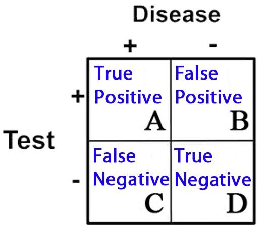
2 X 2 Contingency Table = A 2 X 2 (2 by 2) grid that is created to display the results of a comparison between two categories, e.g. an investigational subject (“test” group) and a gold standard (which determines, for example, who has and does not have disease). There are four possible results in a 2 X 2 table and they are as follows:

True Positives = Subjects in the study that tested positive for a disease that in fact had the condition
True Negatives = Subjects that tested negative for a disease that in fact did not have the condition
False Positives = Subjects that tested positive for a disease that in fact did not have the condition
False Negatives = Subjects that tested negative for a disease that in fact did have the condition

These categories are displayed in 2 X 2 grid as follows:

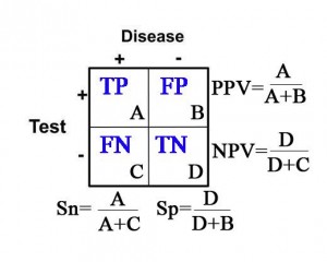
Sensitivity (Sn) = In the group of patients that have disease (the “+” column under “Disease”), it is the proportion of patients with a positive test as it compares to all of the patients with disease. Specifically, it is the true positive rate as it compares to the sum of all of the true positives and false negatives.

Sn= (true positives)/(true pos’s + false neg’s)= A/(A+C)

In other words, sensitivity is the probability that the test result will be positive when the disease is present.

Specificity (Sp) = In the group of patients that do not have disease (the “–” column under “Disease”), it is the proportion of patients with a negative test as it compares to all of the patients without disease. Specifically, it is the true negative rate as it compares to the sum of all of the true negatives and false positives.

Sp= (true negatives)/(true neg’s + false pos’s)= D/(D+B)

In other words, specificity is the probability that the test result will be negative when the disease is not present.

Positive Predictive Value (PPV) = The probability that the patient has disease when the test is positive (the “+” row for “Test”).

PPV=(true postives)/(true pos’s + false pos’s)= A/(A+B)

Negative Predictive Value (NPV) = The probability that the patient does not have disease when the test is negative (the “-” row for “Test”).

NPV= (true negatives)/(true neg’s + false neg’s)=D/(D+C)

Calculations for Sn, Sp, PPV, and NPV are depicted in the table below:

Likelihood Ratio(LR) = This concept incorporates the use of sensitivity and specificity to determine the likelihood that a test will effectively yield the probability of the presence or absence of a disease state or condition. LR’s are utilized to provide a quantitative value in performing a particular test.

Number Needed to Treat (NNT) = The number of patients that need to receive a particular therapy until one is likely to experience benefit from this therapy: e.g.

the number of men over the age of 60 that need to take an aspirin per day until we see one less heart attack (compared to the population of men over 60 not taking aspirin).

Number Needed to Harm (NNH) = NNT is also used to measure harm. The number of patients that need to receive a particular therapy until you are likely to see one harmful event occur is called the Number Needed to Treat to Harm, or NNTH: e.g. the number of men over the age of 60 that need to take an aspirin per day until we see one patient sustain a bleeding stomach ulcer (compared to the population of men over 60 not taking aspirin).

Risk Ratio and Odds Ratio (RR and OR) = Both of these terms refer to the chance of an outcome between 2 groups. They are calculated similarly, but not exactly the same, and typically draw the same general conclusion. The Risk Ratio (RR), also called “Relative Risk,” is a percentage of chance. The OR is based on “odds” and not percent. These concepts will be described in greater detail later in this chapter and in the appendices.

Probability = In essence this is what statistics is all about: the likelihood or chance that a certain outcome will result. Probability is typically expressed as a fraction or percentage.

Population = Reference to all people, or at least all of those with a particular condition.

Sample = It is typically not possible or practical to study an entire population; for that reason, researchers typically study some proportion of individuals in this population. With appropriate sampling (i.e. elimination of bias), there is the greatest chance that the conclusion drawn will represent the entire population.

Bias = Whether intentional or not, it is the unfair favoritism of one particular outcome over another. Some of the common types of bias in medical literature are:

Selection Bias = typically the result of a non-randomized or poorly randomized study

Publication Bias = Pharmaceutical companies are frequently accused of this: e.g. only publishing “positive” studies, i.e. those that reveal their drug is beneficial. In contrast, they may not publish studies that are not favorable for their particular drug.

Surveillance Bias (aka. Detection Bias) = When one group of patients is

followed more closely in a study than another group. This typically happens because one group is considered to be more sick or more of interest by the investigators because they are the study group and not the placebo group.

Information (Recall) Bias = When information is gathered by way of the patient’s recollection of events, errors can occur because the patient may not recall pertinent details. This type of bias can also occur when there isn’t consistency in how questions are asked of patients: patients may give different answers depending on how they are asked questions. This is the classic, “garbage in, garbage out” error.

Spectrum Bias = Occurs when patients are studied at different points in their disease course: e.g. early vs. late appendicitis, patients have different likelihoods of positive findings on radiologic imaging.

Confounders = Results may be skewed in a study because of factors that the investigators didn’t account for. This type of error can give a false impression of cause and effect: e.g. immunization rates among kids have increased since the 1970’s and the rate of autism has increased since the 1970’s. Conclusion: Immunizations cause autism. In fact, there are many confounders: change in definition of autism to autism-spectrum disorder, better detection of autism, and many others.

Null hypothesis = The assumption that there is no difference between groups being studied.

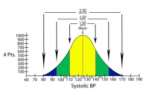
Normal distribution of data = The typical “bell shaped curve” that results when there is a normal distribution of data around the mean.

Standard deviation = Quantifies the distribution of data around some average value: e.g. the second standard deviation from the mean identifies about 95% of values measured, and does not include the roughly 5% of measured values that remain (in medicine, these latter values would be considered to be significantly different from the mean or average).

Statistical significance = The point at which, or the range of values outside of which, an event is not likely to have occurred by chance alone. Statistical significance establishes what is accepted to be a true difference between two groups (e.g. therapy 1 is better than therapy 2). Statistical significance is most commonly determined in one of two ways in the medical literature: either by p-values or confidence intervals.

p-value = p stands for “probability. It is the point at which statistical significance is defined. In other words, the point at which it is accepted that a difference between two groups is not due to chance. Traditionally the most common measure of statistical significance in medical literature, the p-value is typically set at 0.05. This means that there is a 5% probability (or less) that the results obtained in a study are due to chance alone: or stated another way, if the study were performed again, there is a 5% (or less) probability that the result would be outside the cutoff point of the p-value.

Confidence interval = In a comparison of populations, it is a range of statistical values (e.g. means, or LR’s) within which the “true result” is likely to reside. Confidence intervals are used to reveal the reliability of an estimate, and is typically set at 95%. This means that if the study were repeated 100 times, we would expect the result to fall within this range on 95 of those trials.

Bayesian Analysis or Bayes’ theorem = This is a form of deductive reasoning; that is to say, the clinician subjectively determines the probability of a particular event (prior probability), then performs a test that has some known likelihood of supporting or refuting that belief. In the end, then, the clinician draws a conclusion, posterior probability, and determines if the result is sufficient or if more testing needs to be done.

Explanation of Statistical Terms and Concepts Used in the Diagnosis of Disease:

Sensitivity and Specificity:

Arguably two of the most important statistical concepts that a physician (or other medical provider) needs to understand in order to perform a critical review of medical literature are sensitivity and specificity. In a perfect world with a perfect study, a test would be positive only when disease is present and negative only when there is absence of disease. Let’s imagine a study in which we are evaluating the reliability of a test to determine the presence of pancreatitis (inflammation of the pancreas) in 1000 patients with abdominal pain. Let’s imagine that the study results turned out as they are illustrated below.

The results of this study reveal that there are 500 patients with abdominal pain that did not have pancreatitis and 500 patients with abdominal pain that did have pancreatitis (based on some kind of “gold standard” such as a CT scan). In this study, it was found that by using the investigational lab test, a lipase level, you could accurately diagnose pancreatitis when the level was greater than 300 units. Conversely, all patients with a level less than 300 were found to not have pancreatitis. This would be illustrated as below in a 2 X 2 contingency table.

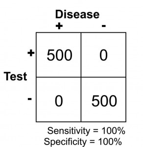
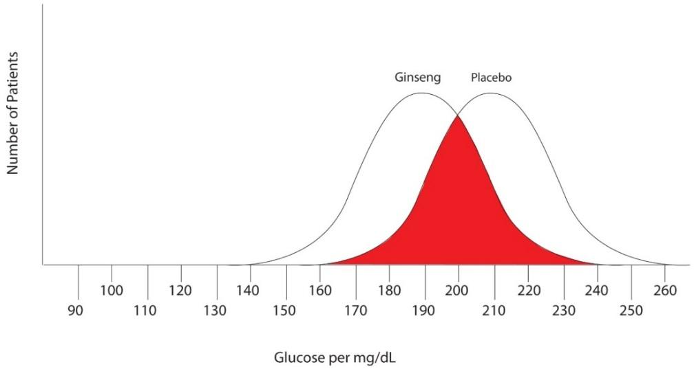
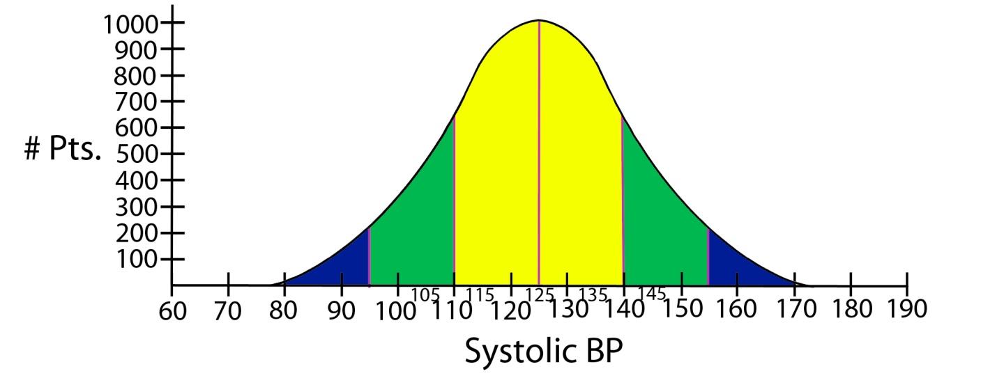
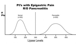
Note that there are no false negatives and no false positives, thus the test has 100% sensitivity and specificity. A more common scenario is the situation in which there is overlap of results, in that some patients without disease that have an extreme result will be found to have disease based on a test (false positives) and some patients with disease will be found to not have a positive test (false negatives). Imagine the study illustrated below in which investigators are looking to diagnose the presence of diabetes based on the results of a blood (serum) glucose level 2 hours after eating a standardized meal (postprandial glucose check). Imagine that researchers checked 500 people with and 500 people without diabetes (disease determined again by some accepted gold standard), and came up with the following results.

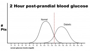
Notice that there is a wide range of glucose levels in both diabetic and non-diabetic patients at 2 hours after eating. Notice, as well, that there are cut-offs that define normal and abnormal. Where we choose these cut-offs to be determines the sensitivity and specificity of this test. To maximize both sensitivity and specificity, and get the overall best accuracy for this test, we choose a cut-off that is in the middle, where our two populations intersect.

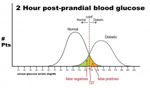
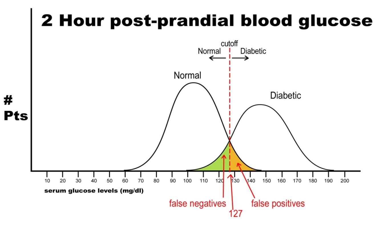
In this case, any patient with a serum glucose level greater than or equal to 127 (the middlemost value) at 2 hours postprandial would be labeled as diabetic, and any patient with a serum glucose level of less than 127 would be labeled non-diabetic. This would yield the following results:

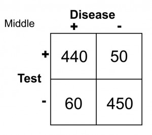
Sn = 440/(440 + 60) = 0.88 or 88%

Sp = 450/(450 + 50) = 0.90 or 90%

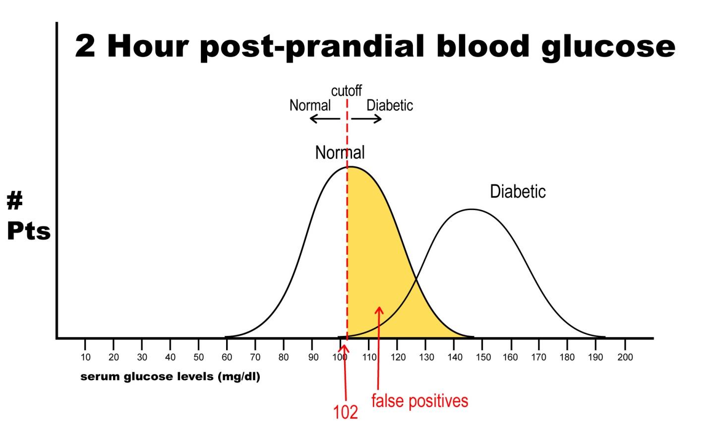
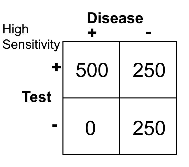
Let’s say, now, that it is vital that this test be 100% sensitive so that we do not miss any patients that could potentially have diabetes. If we move the cut-off to a glucose level of 102, then we get the following results:

Notice that there are no false negatives and thus 100% sensitivity. Notice as well, however, that the number of false positives has increased dramatically. This change in cut-off value would yield the following results:

Sn = 500/(500 + 0 ) = 1.0 or 100

Sp = 250/(250 + 250) = 0.50 or 50%

Notice that by choosing this cut off point the test does exceedingly well at identifying patients with disease. In changing to this cut off point, however, the number of false positives increases substantially, so we are now going to identify many people as having disease when they really do not have it (has low specificity). Notice further, though, that because a highly sensitive test has a low false negative rate, when the test is negative, it virtually rules out disease (i.e. a negative result in a highly sensitive test means the patient does not have disease).

Finally, let’s imagine that we need to have 100% specificity with this screening test because we are going to expose the patient to a treatment that could be deleterious to non-diabetics. If we change the postprandial glucose cut-off to a level of 148 as the definition of diabetes, then we get the following results:

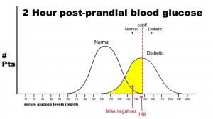
In this case, there are no false positives, but 250 false negatives. This yields the following results:

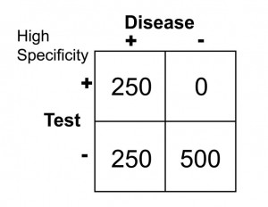
Sn = 250/(250 + 250) = 0.50 or 50%

Sp = 500/(500 + 0) = 1.0 or 100%

This selected cut off point makes this test exceedingly good at identifying patients without diabetes, but it is also labeling a lot of people as non-diabetic when they really have disease (the false negative rate increased as we increased the specificity). Notice in this case, though, that when the test is positive in a highly specific case that this virtually assures that the person does have disease: i.e. when the person’s blood sugar, in this example, is greater than 148 mg/dl, the person is essentially certain to have diabetes.

Positive and negative predictive values:

As stated previously, PPV is the probability that the disease is present when the test is positive, and the NPV is the probability that the disease is not present when the test is negative. With PPV and NPV, we are now dealing with how well a test performs. Predictive values, however, can change dramatically as the prevalence of disease changes from one population studied to another. If bias and confounders are not introduced, sensitivity and specificity do not change from one study to another despite a change in prevalence of disease. To illustrate this point, imagine the following study results.

A health system studies the efficacy of having housekeeping staff collect throat swabs on patients, as a cost saving measure, instead of having nurses perform the swabbing of the patient’s throat (the gold standard). Investigators perform 2 studies evaluate patients for Strep throat. In the first study, investigators enroll patients that have a sore throat, fever, and exudate (pus) on the tonsils. In this study, 50% of patients are found to have Strep throat by the “gold standard.” In the next study, investigators evaluate patients with sore throat, fever, and no exudate. In this case, using a gold standard, the prevalence of disease (proportion of patients found to have Strep throat) is found to be only 1%. The sensitivity this test when housekeepers obtain the specimens is 20% and the specificity is 95% (meaning that the housekeeping staff are not too good compared to nurses when it comes to swabbing the tonsils for Strep, but when they did swab the tonsils they did it right in that they did not have many false positives). In both cases, the Sn and Sp are the same, 20% and 95% respectively. The results obtained are below. Before looking at the answer, calculate the PPV and NPV for each study.

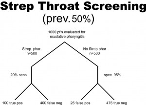
PPV = 100/(100 + 25) = 0.80 or 80%

NPV = 475/(475 + 400) = 0.54 or 54%

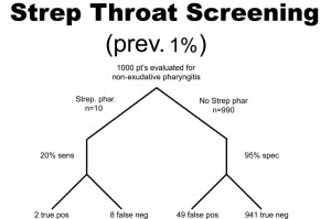
PPV = 2/(2 + 49 )= 0.039 or 3.9%

NPV = 941/(941 + 8) = 0.99 or 99%

So, what can we glean from these studies? Well, first of all, the housekeepers seem to have a very poor ability to obtain proper specimens compared to nurses (if we accept their results as the gold standard) since the sensitivity is only 20% in each study (i.e. there are a lot of false negatives). In other words, this study reveals that patients with disease were not diagnosed 80% of the time because the specimen was not collected as well as if it had been collected by the nurse, but why would we expect a housekeeper to know how to do this task? Notice, though, that the PPV for the test is actually pretty high, at 80%, when there is a high prevalence of disease. That is because PPV tends to track with Sp as they both share “false positives” in their calculation. Notice that the NPV is actually pretty poor when there is a high prevalence of disease, but it is very high when there is a low prevalence of disease. Can you see why this is the case? Notice that with a prevalence of only 1%, 99% of patients do not have disease. That being the case, if you didn’t do the test at all and just picked a patient randomly from this population as not having disease, you’d be correct 99% of the time. We can conclude for this study that having the housekeepers obtain specimens for Strep screening appears to be a bad idea.

Likelihood Ratio (LR)

Likelihood ratios are used when assessing the likelihood of a disease being present based on a certain test. Sensitivity and specificity are used in the calculation of LR’s. By helping to determine the usefulness of a test, LR’s predict the chance that a particular disease state exists. LR is a term commonly seen in modern medical literature because it provides very practical and useful information as you look to counsel individual patients regarding a particular test.

LR+ is for “ruling in disease” (determining disease is present).

LR- is for “ruling out disease” (determining disease is not present).

The calculations are as follows:

LR+ = sensitivity/(1-specificity)

We call this LR+, or positive likelihood ratio, because it is the likelihood that the person has a particular diagnosed condition. There is also a negative likelihood ratio, or LR-, which indicates the likelihood that someone does not have a particular condition. It is calculated by means of the following:

LR- = (1-sensitivity)/specificity

Likelihood ratios yield results that range from 0 to infinity:

LR range: 0———-1———-2———-//———-10—-infinity

Whether talking about LR+ or LR-, if the LR value is 1, it means this is a neutral value. That means it gives no indication as to the usefulness of the test. If a study is done where LR+ = 1, that means that when the test is positive the patient is just as likely to have disease as not have disease. If the calculated LR+ is found to be greater than 5 but still less than 10, the test in question is considered to be moderately useful in its predictive ability for determining the presence of disease. If the LR+ is greater than 10, it is considered very useful in determining the presence of disease. If the LR- is calculated to be less than 0.2 (1/5), then the test is considered moderately useful in determining the absence of disease. If the LR- is less than 0.1, it is considered very useful. The higher the LR+ is and the lower the LR- is, the more useful the test is. So, to interpret the value of LR+, for example, if a test is found to have LR = 5, that means that a patient with a positive result is 5 times more likely to have the disease being tested than not to have the disease. For more explanation about LR’s, and for more examples and calculations, see appendix 5a.

Case scenario

A 50 year old woman presents to your internal medicine office with a headache. She has had this waxing and waning headache for the past 12 weeks and is concerned because she has a friend that had a similar headache and the “Lyme disease specialist” that she saw determined it was the result of chronic Lyme disease. The patient wants to receive antibiotics to treat this presumed Lyme related headache. The patient doesn’t want to waste her time with testing for Lyme because, “the tests are inaccurate.” In your evaluation of her you discover that she does spend a fair amount of time in the outdoors but hasn’t been camping and doesn’t recall ever having a tick bite or a rash. You inform her that you think she is at very low risk for Lyme disease and thus unlikely to have any kind of Lyme related headache. You concede that the accuracy of the test is not perfect but that the CDC (Centers for Disease Control) reports the test to be 80% sensitive and 90% specific for diagnosing Lyme disease. Should this patient receive antibiotics for Lyme disease without any testing? If a Lyme test is performed and found to be negative, what is the negative predictive value of this test?

Natural Science Module EBM

Evidence Based Medicine

Facts are the air of scientists. Without them you can never fly.*

Linus Pauling

Introduction:

“Medicine is both an art and a science.” This statement is not just a cliché. The art of medicine is the ability of the physician to collect information from a patient, interpret it, and tailor treatment that best suits the individual’s needs. The science of medicine is choosing the most effective treatment based on the best medical literature available. As a physician, or other health care provider, you will spend countless hours poring over journal articles and partaking in continuing medical education in an effort to help your patients: and, of course, to maintain your licensure and board certification. Studying EBM may seem like a departure from clinical medicine, as we have studied it so far in this text, but in fact it actually defines how one diagnoses and treats disease. Reviewing medical literature will be a big part of the rest of your life as you practice evidence based medicine.